How to make a link in exile

Links are one of the main tools when working in Microsoft Excel. They are an integral part of the formulas that apply in the program. Other of them serve to go to other documents or even resources on the Internet. Let's find out how to create various types of referring expressions in Excele.

Creating various types of links

Immediately, it should be noted that all referring expressions can be divided into two large categories: intended for calculations as part of formulas, functions, other tools and employees to go to the specified object. The latter is still called hyperlinks. In addition, links (links) are divided into internal and external. Internal is the referring expressions inside the book. Most often, they are used for calculations, as an integral part of the formula or argument of the function, indicating a specific object where the data being processed is contained. In the same category, you can attribute those that refer to the place on another sheet of the document. All of them, depending on their properties, are divided into relative and absolute.

External links refer to an object that is outside the current book. It may be another Excel book or place in it, a document of another format and even the site on the Internet.

From what type of type you want to create, and the selectable method of creation depends. Let's stop at various ways in more detail.

Method 1: Creating references in the formulas within one sheet

First of all, consider how to create various options for references for formulas, functions and other Excel calculation tools within one sheet. After all, they are most often used in practice.

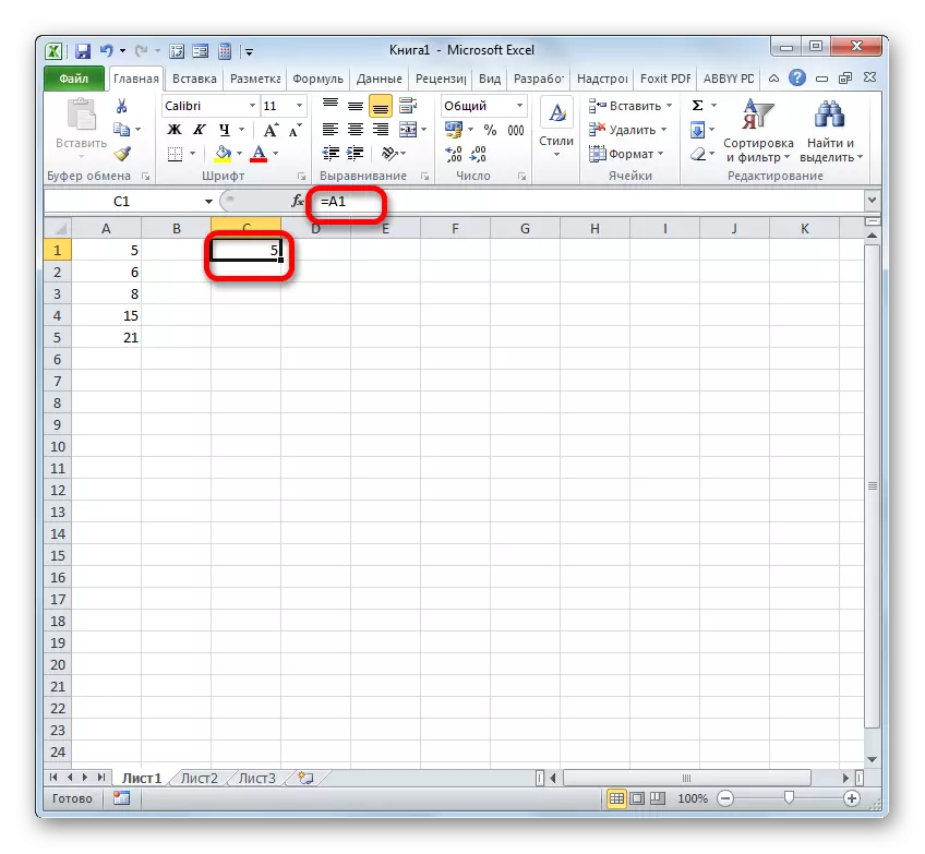
The simplest reference expression looks like this:

= A1.

The mandatory attribute of the expression is the sign "=". Only when installing this symbol in the cell before expression, it will be perceived as referring. The obligatory attribute is also the name of the column (in this case a) and the column number (in this case 1).

The expression "= A1" suggests that the element in which it is installed, data from the object with the coordinates A1 is tightened.

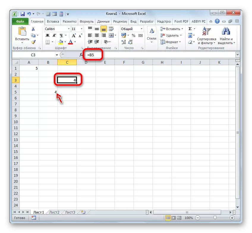
If we replace the expression in the cell, where the result is displayed, for example, on "= b5", the values ​​from the object with the coordinates B5 will be tightened.

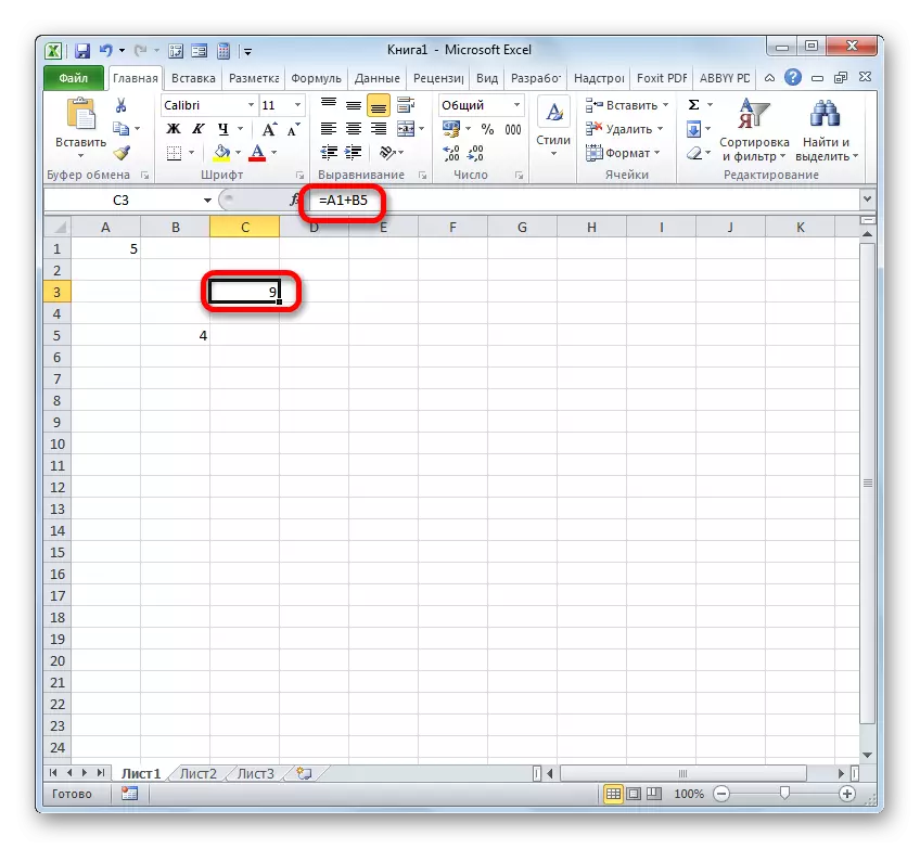
Using links, various mathematical actions can also be performed. For example, we write down the following expression:

= A1 + B5

Clause on the ENTER button. Now, in the element where this expression is located, summation of the values ​​that are placed in objects with coordinates A1 and B5 will be made.

By the same principle, division is made, multiplying, subtraction and any other mathematical action.

To record a separate link or as part of the formula, it is not necessary to drive it away from the keyboard. It is enough to install the symbol "=", and then put the left mouse button along the object to which you want to refer. His address will be displayed in the object where the "equal" sign is installed.

But it should be noted that the coordinate style A1 is not the only one that can be used in the formulas. In parallel, the Excel works the R1C1 style, in which, in contrast to the previous version, the coordinates are indicated by letters and numbers, but exclusively by numbers.

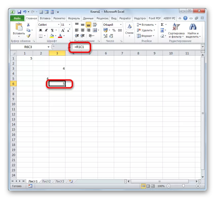
The expression R1c1 is equivalent to A1, and R5C2 - B5. That is, in this case, in contrast to the style of A1, the coordinates of the line are in the first place, and the column is on the second.

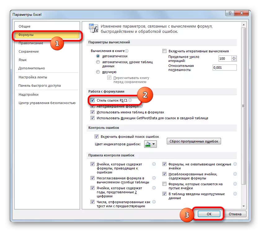
Both styles act in Excel is equivalent, but the default coordinate scale has the form A1. To switch it to the R1C1 view, you are required in the Excel parameters in the Formulas section, check the checkbox opposite the R1C1 Link Style item.

After that, on the horizontal coordinate panel, figures will appear instead of letters, and the expressions in the formula row will acquire the form R1C1. Moreover, the expressions recorded not by making coordinates manually, and the click on the appropriate object will be shown as a module with respect to the cell in which it is installed. In the image below it is a formula

= R [2] C [-1]

If you write an expression manually, then it will take the usual view R1C1.

In the first case, the relative type was presented (= R [2] C [-1]), and in the second (= R1c1) - absolute. Absolute links refer to a specific object, and relative - to the position of the element, relative to the cell.

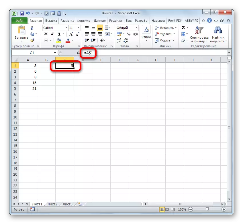
If you return to the standard style, then the relative links have the form A1, and the absolute $ a $ 1. By default, all references created in Excel are relative. This is expressed in the fact that when copying with a filling marker, the value in them changes relative to the move.

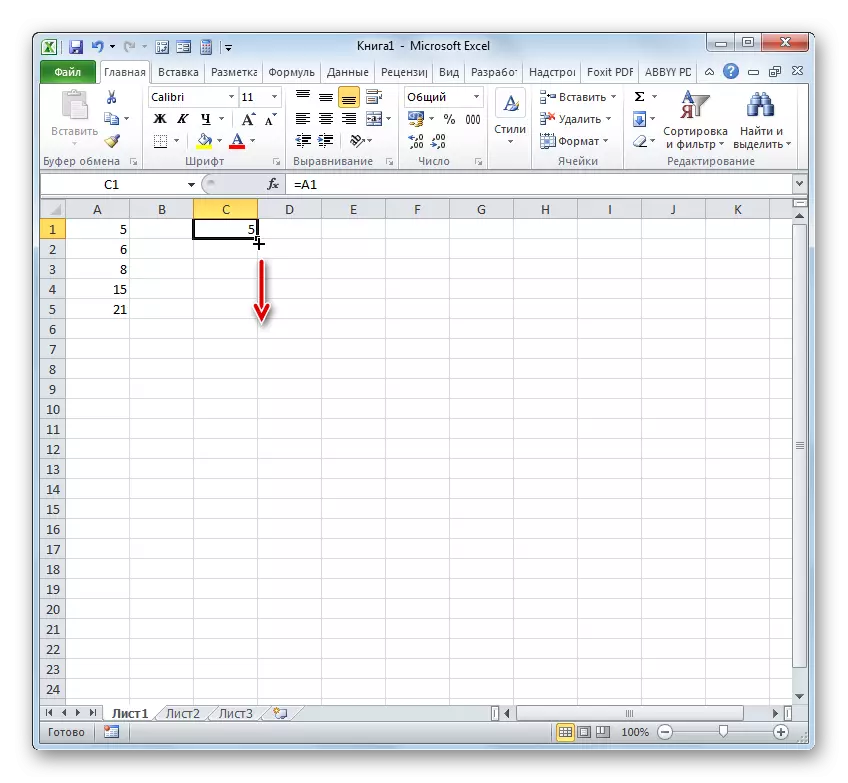
1. To see how it will look in practice, weave to the cell A1. We install in any empty leaf element the symbol "=" and clay on the object with the coordinates A1. After the address is displayed as part of the formula, clay on the ENTER button.



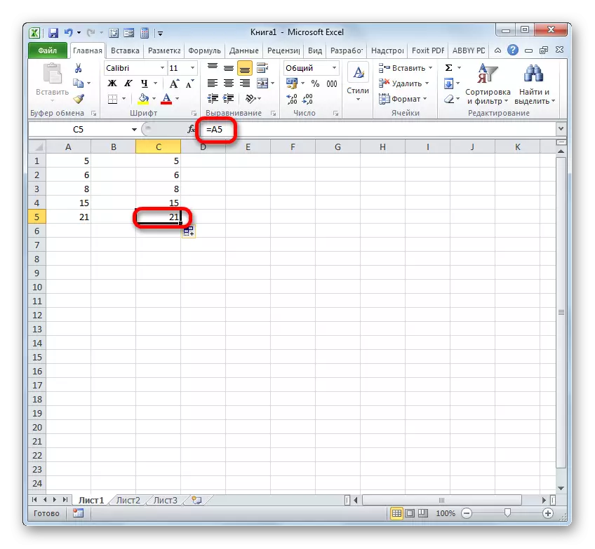
2. We bring the cursor to the lower right edge of the object, in which the result of the formula processing appeared. The cursor is transformed into the fill marker. Click the left mouse button and stretch the pointer parallel to the data with the data you want to copy.



3. After the copying was completed, we see that the values ​​in subsequent range elements differ from the one in the first (copied) element. If you select any cell where we copied the data, then in the formula row you can see that the link has been changed relative to the move. This is a sign of its relativity.

The relativity property sometimes helps a lot when working with formulas and tables, but in some cases you need to copy the exact formula unchanged. To do this, the link is required to transform into absolute.

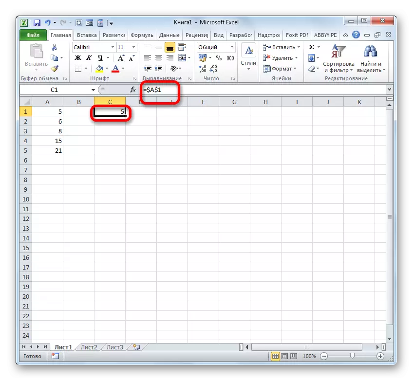
1. To carry out the transformation, it is enough about the coordinates horizontally and vertically put a dollar symbol ($).



2. After we apply a fill marker, you can see that the value in all subsequent cells when copying is displayed exactly the same as in the first one. In addition, when you hover on any object from the range below in the formula string, it can be noted that the links remained completely unchanged.

In addition to absolute and relative, there are still mixed links. The dollar sign marks either only column coordinates (example: $ A1),

either only the coordinates of the string (example: A $ 1).

The dollar sign can be done manually by clicking on the appropriate symbol on the keyboard ($). It will be highlighted if in the English keyboard layout in the upper case click on the "4" key.

But there is a more convenient way to add the specified symbol. You just need to highlight the reference expression and press the F4 key. After that, the dollar sign will appear simultaneously in all coordinates horizontally and vertical. After re-pressing on the F4, the link is converted to mixed: the dollar sign will only remain in the coordinates of the line, and the column coordinates will disappear. Another Pressing F4 will result in the opposite effect: the dollar sign will appear at the column coordinates, but the row coordinates will disappear. Further, when pressing the F4, the link is converted to the relative without dollars. The following press turns it into absolute. And so on a new circle.

In Excel, you can refer not only to a specific cell, but also on a whole range. The address of the range looks like the coordinates of the upper left element and the lower right, separated by the colon sign (:). For example, the range allocated in the image below has coordinates A1: C5.

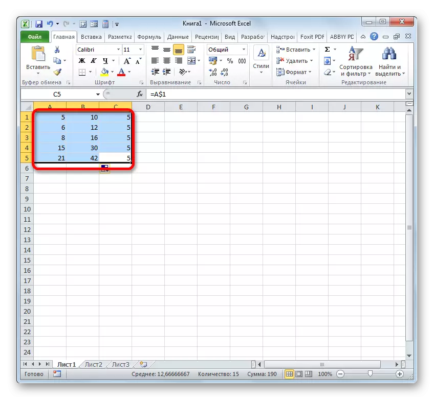
Accordingly, the link on this array will look like:

= A1: C5

Lesson: Absolute and Relative Links to Microsoft Excel

Method 2: Creating references in the formulas for other sheets and books

Prior to that, we considered actions only within one sheet. Now let's see how to refer to the place on another sheet or even the book. In the latter case, it will not be internal, but an external link.

The principles of creation are exactly the same as we viewed above when actions on one sheet. Only in this case will need to specify an additional leaf address or book where the cell or the range is required to refer to.

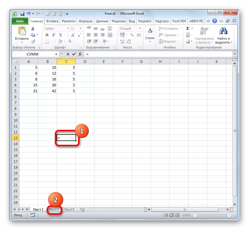
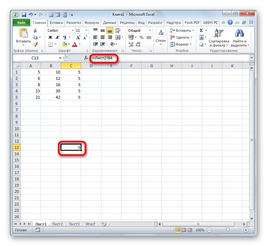
In order to refer to the value on another sheet, you need to specify its name between the "=" sign and the coordinates of the cell, then install an exclamation mark.

So the link on the cell on a sheet 2 with the coordinates of B4 will look like this:

= List2! B4

The expression can be driven by hand from the keyboard, but it is much more convenient to do as follows.

1. Install the "=" sign in the item that will contain a reference expression. After that, using a shortcut above the status bar, go to that sheet where the object is located to refer to.



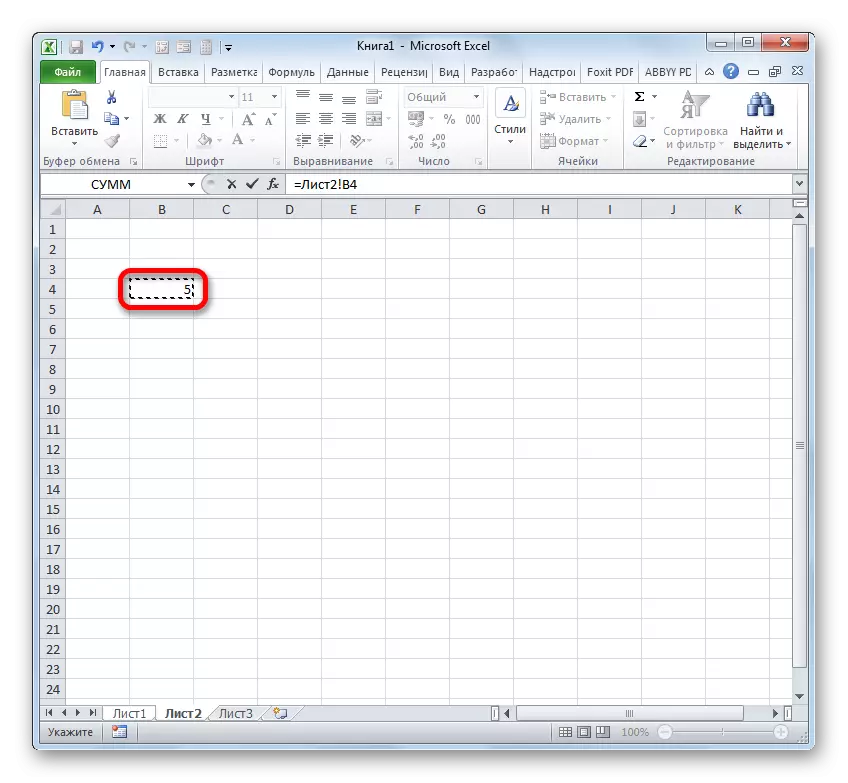
2. After the transition, select this object (cell or range) and click on the ENTER button.



3. After that, there will be an automatic return to the previous sheet, but the reference we need will be formed.

Now let's figure out how to refer to the element located in another book. First of all, you need to know that the principles of operation of various functions and Excel tools with other books differ. Some of them work with other Excel files, even when they are closed, while others require mandatory launch of these files.

In connection with these features, the type of link on other books is different. If you introduce it to a tool that works exclusively with running files, then in this case you can simply specify the name of the book you refer to. If you intend to work with a file that are not going to open, then in this case you need to specify the full path to it. If you do not know, in what mode you will work with the file or not sure how a specific tool can work with it, then in this case, again, it is better to specify the full path. Even it will definitely not be.

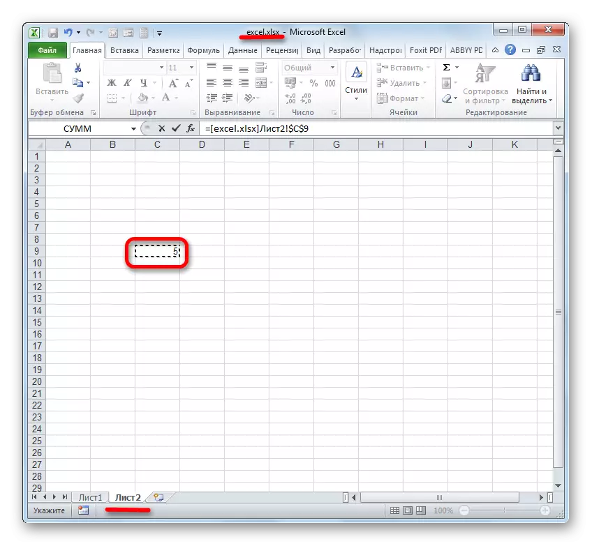
If you need to refer to an object with the address C9, located on a sheet 2 in the running book called "excel.xlsx", then you should record the following expression in the sheet element where the value will be displayed:

= [Excel.xlsx] list2! C9

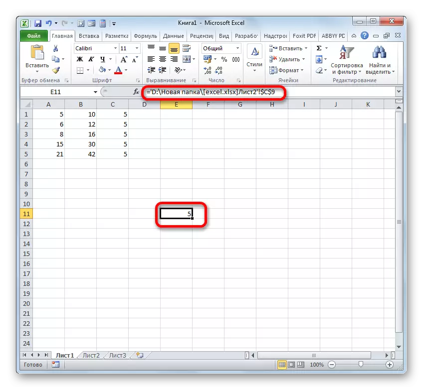
If you plan to work with a closed document, then, among other things, you need to specify the path of its location. For example:

= 'D: \ New folder \ [Excel.xlsx] sheet2'! C9

As in the case of creating a reference expression to another sheet, when creating a link to the element another book, you can, how to manually enter it, and do it by selecting the corresponding cell or range in another file.

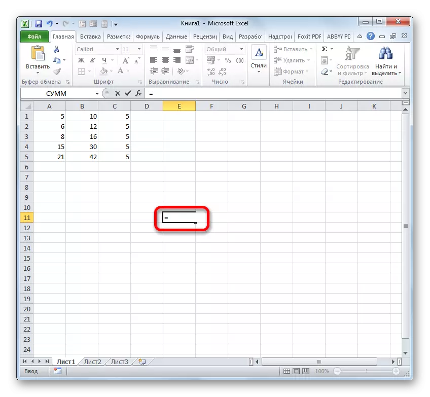
1. We put the character "=" in the cell where the referring expression will be located.



2. Then open the book to which you want to refer if it is not running. Clay on her sheet in the place that you want to refer to. After that, click on ENTER.



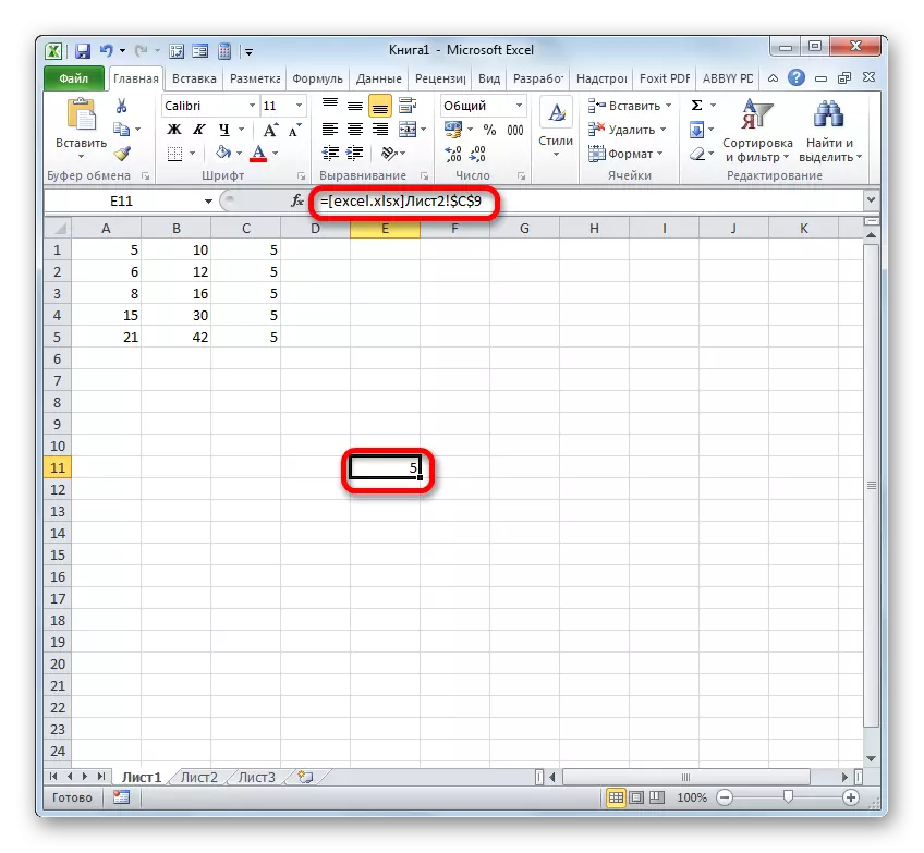
3. There is an automatic return to the previous book. As you can see, it has already mastered the link to the element of that file, by which we clicked in the previous step. It contains only the name without a way.



4. But if we close the file to refer to, the link will immediately transform automatically. It will present the full path to the file. Thus, if a formula, a function or tool supports work with closed books, now, thanks to the transformation of the reference expression, it will be possible to take this opportunity.

As you can see, the lifting link to the element of another file using click on it is not only much more convenient than the enclosure of the address manually, but also more universal, since in that case the link itself is transformed depending on whether the book is closed to which it refers, Or open.

Method 3: Function Two

Another option to refer to the object in Excel is the use of the function of the dash. This tool is just intended to create reference expressions in text form. The references created thus are also called "superable", since they are connected with the cell that specified in them is even more tight than typical absolute expressions. The syntax of this operator:

= DVSSL (link; A1)

"Link" is an argument that refers to a cell in text form (wrapped with quotes);

"A1" is an optional argument that determines which style coordinates are used: A1 or R1C1. If the value of this argument is "Truth", then the first option is used if "lies" is the second one. If this argument is generally omitted, then by default it is believed that the addressing of type A1 is applied.

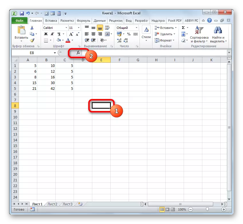
1. We note the element of the sheet in which the formula will be. Clay on the "Insert function" icon.



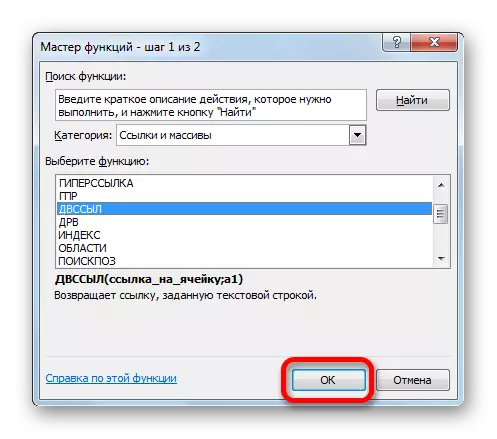
2. In the wizard of the functions in the "Links and Arrays" block, we celebrate "DVSSL". Click "OK".



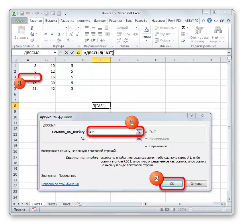
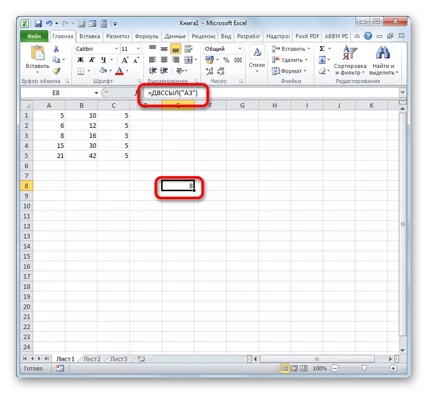
3. The arguments window of this operator opens. In the "Link to the cell" field, set the cursor and highlight the click of the mouse that the element on the sheet to which we want to refer to. After the address is displayed in the field, "wrapping" with its quotes. The second field ("A1") is left blank. Click on "OK".



4. The result of processing this function is displayed in the selected cell.

In more detail, the advantages and nuances of the DVRSL function are considered in a separate lesson.

Lesson: Function Dultnsil in Microsoft Excel

Method 4: Creating a hyperlink

The hyperlinks differ from the type of links that we considered above. They do not serve to "pull up" data from other areas in that cell, where they are located, and in order to make the transition when clicking in the area to which they refer.

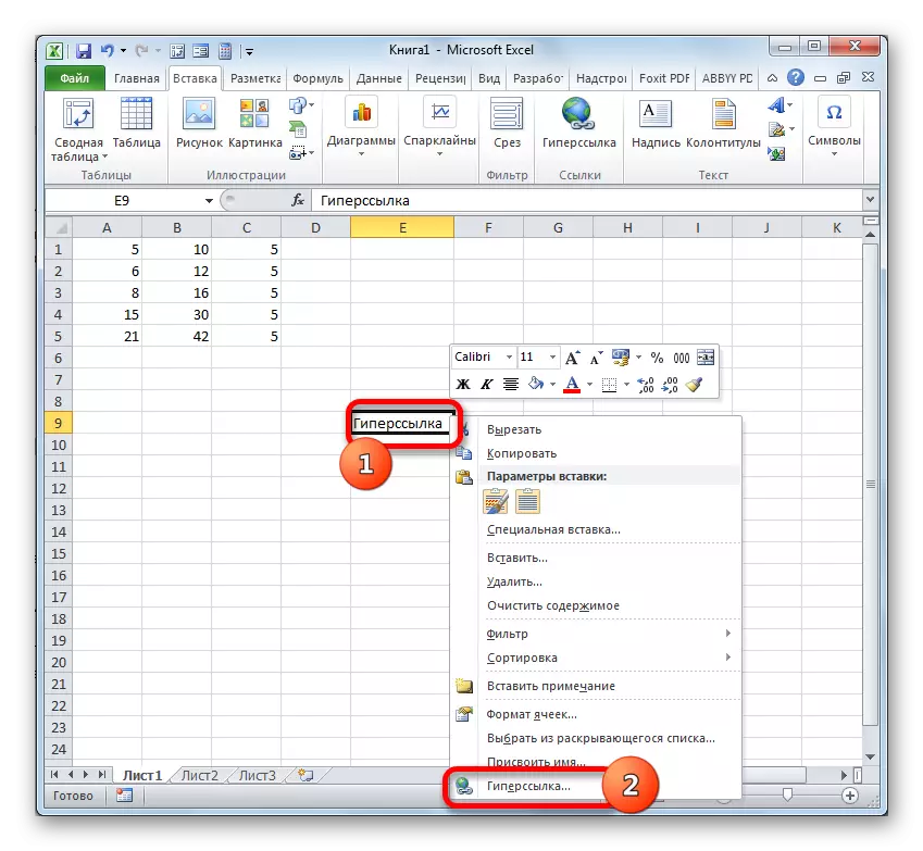
1. There are three options for switching to the window of creating hyperlinks. According to the first of them, you need to highlight the cell into which the hyperlink will be inserted, and click on it right mouse button. In the context menu, select the option "Hyperlink ...".

   

   Instead, you can, after selecting an item where the hyperlink is inserted, go to the "Insert" tab. There on the ribbon you need to click on the "Hyperlink" button.

   

   Also, after selecting the cell, you can apply the Ctrl + K keys.

2. After applying any of these three options, the Hyperlink Creation window opens. In the left part of the window, there is a choice of, with which object it is required to contact:
   • With a place in the current book;
   • With a new book;
   • With a website or file;
   • With e-mail.



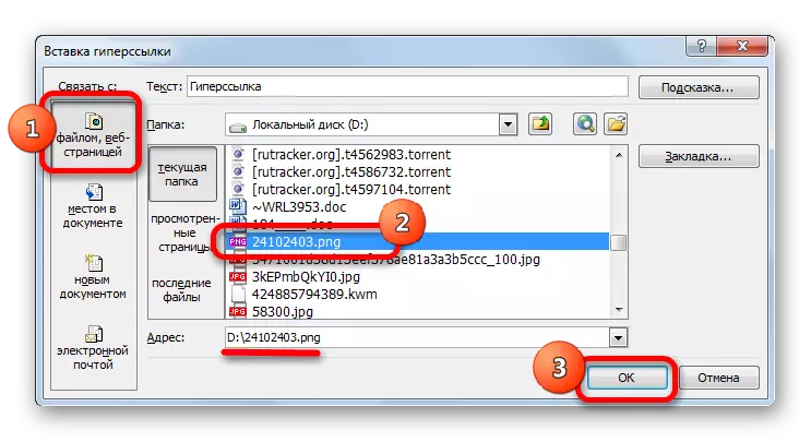
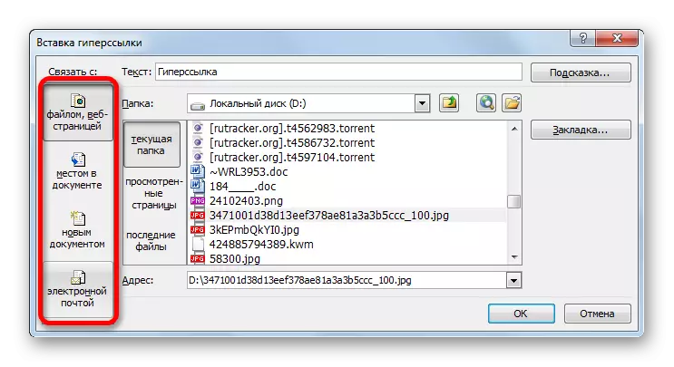
3. By default, the window starts in communication mode with a file or web page. In order to associate an element with a file, in the central part of the window using the navigation tools, you need to go to that directory of the hard disk where the desired file is located and highlight it. It can be both an Excel book and a file of any other format. After that, the coordinates will be displayed in the "Address" field. Next, to complete the operation, click on the "OK" button.

   

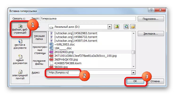
   If there is a need to communicate with the website, then in this case, in the same section of the menu creation window in the "Address" field you need to simply specify the address of the desired web resource and click on the "OK" button.

   

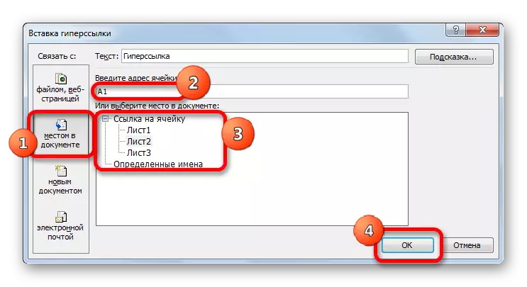
   If you want to specify a hyperlink to a place in the current book, you should go to the "Tie with the place in the document" section. Next, in the central part of the window, you need to specify the sheet and the address of the cell from which the connection should be made. Click on "OK".

   

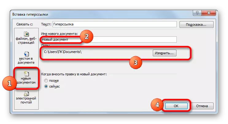
   If you need to create a new Excel document and bind it using a hyperlink to the current book, you should go to the section "Tie with a new document". Next, in the central area of ​​the window, give it a name and specify its location on the disk. Then click on "OK".

   

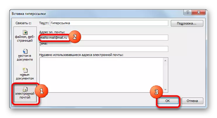
   If you wish, you can connect the leaf element with a hyperlink even with email. To do this, we move to the "Tie with Email" section and in the "Address" field indicate E-mail. Clay on "OK".



4. After the hyperlink was inserted, the text in the cell in which it is located, the default becomes blue. This means that the hyperlink is active. To go to the object with which it is connected, it is enough to double-click on it with the left mouse button.

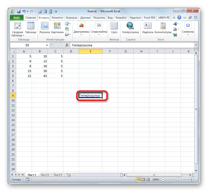
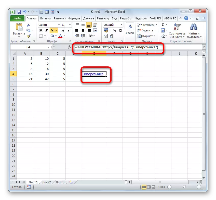
In addition, the hyperlink can be generated using an embedded function having a name that speaks for itself - "hyperlink".

This operator has syntax:

= Hyperlink (address; name)

"Address" - an argument that indicates the address of the website on the Internet or file on the hard drive, with which you need to establish communication.

"Name" - an argument in the form of text, which will be displayed in a sheet element containing a hyperlink. This argument is not mandatory. In its absence, the address of the object will be displayed in the sheet element to which the function refers to.

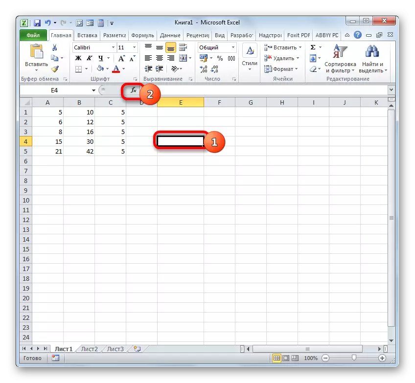
1. We highlight the cell in which the hyperlink will be located, and clay on the "Insert function" icon.



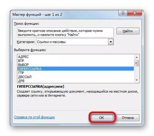
2. In the functions wizard, go to the "Links and Arrays" section. We note the name "hyperlink" and click on "OK".



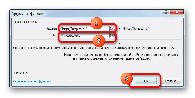
3. In the argument window in the "Address" field, specify the address to the website or file on the Winchester. In the "Name" field we write the text that will be displayed in the sheet element. Clay on "OK".



4. After that, the hyperlink will be created.

Lesson: how to make or remove hyperlinks in Excel

We found out that there are two link groups in Excel tables: used in formulas and employees to transition (hyperlink). In addition, these two groups are divided into many smaller species. It is from a specific type of level and depends on the algorithm for the creation procedure.