Excel list

Creating drop-down lists allows not only to save time when choosing an option in the process of filling out tables, but also to protect yourself from the erroneous making of incorrect data. This is a very convenient and practical tool. Let's find out how to activate it in Excel, and how to use it, as well as find out some other nuances of handling it.

Use of drop-down lists

Following, or as it is customary to speak, the drop-down lists are most often used in the tables. With their help, you can limit the range of values ​​made into the table array. They allow you to choose to make a value of only from a pre-prepared list. This simultaneously speeds up the procedure for making data and protects from an error.

Procedure for creating

First of all, let's find out how to create a drop-down list. It is easiest to do this with a tool called "Data Check".

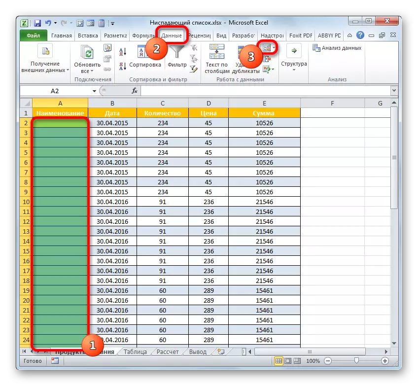
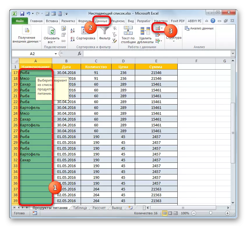
1. We highlight the column of the table array, in the cells of which it is planned to place the drop-down list. Moving into the "Data" tab and clay on the "Data Check" button. It is localized on the ribbon in the "Working with Data" block.



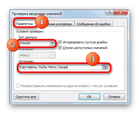
2. The "Verification" tool window starts. Go to the "Parameters" section. In the "Data Type" area from the list, select the "list" option. After that, we move to the field "Source". Here you need to specify a group of names intended for use in the list. These names can be made manually, and you can specify a link to them if they are already posted in Excel in another place.

   If manual entry is selected, then each list item is required to enter into the area over a semicolon (;).

   

   If you want to tighten the data from an existing table array, then you should go to the sheet where it is located (if it is located on the other), put the cursor to the "Source" area of ​​the data verification window, and then highlight the array of cells where the list is located. It is important that each separate cell is located a separate list item. After that, the coordinates of the specified range should be displayed in the "Source" area.

   

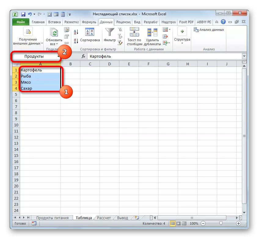
   Another option to install the communication is the assignment of the array with the list of the name. Select the range in which the data values ​​are indicated. To the left of the formula string is the area of ​​names. By default, in it, when the range is selected, the coordinates of the first selected cell are displayed. We are just entering the name for our purposes, which we consider more appropriate. The main requirements for the name is that it is unique within the book, did not have gaps and necessarily began with the letter. Now that the range that we have been identified before this item will be identified.

   

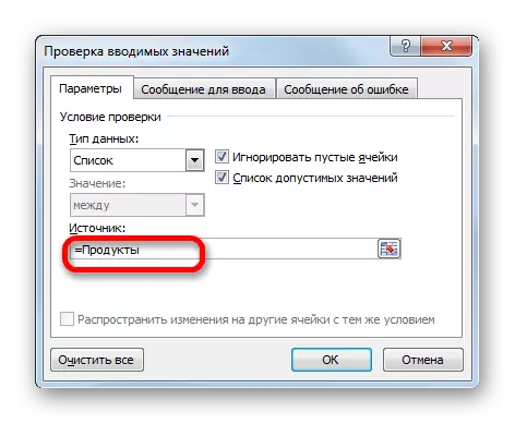
   Now, in the Data Verification window in the "Source" area, you need to install the "=" symbol, and then immediately after it to enter the name we have assigned the range. The program immediately identifies the relationship between the name and array, and will pull the list that is located in it.

   

   But much more efficiently will be used to use the list if you convert to the "smart" table. In such a table, it will be easier to change the values, thereby automatically changing the list items. Thus, this range will actually turn into a substitution table.

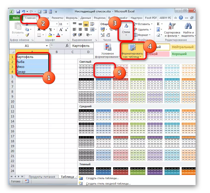
   In order to convert the range into a "smart" table, select it and move it into the Home tab. There, clay on the button "Format as a table", which is placed on the tape in the "Styles" block. A large style group opens. On the functionality of the table, the choice of a particular style does not affect anyone, and therefore choose any of them.

   

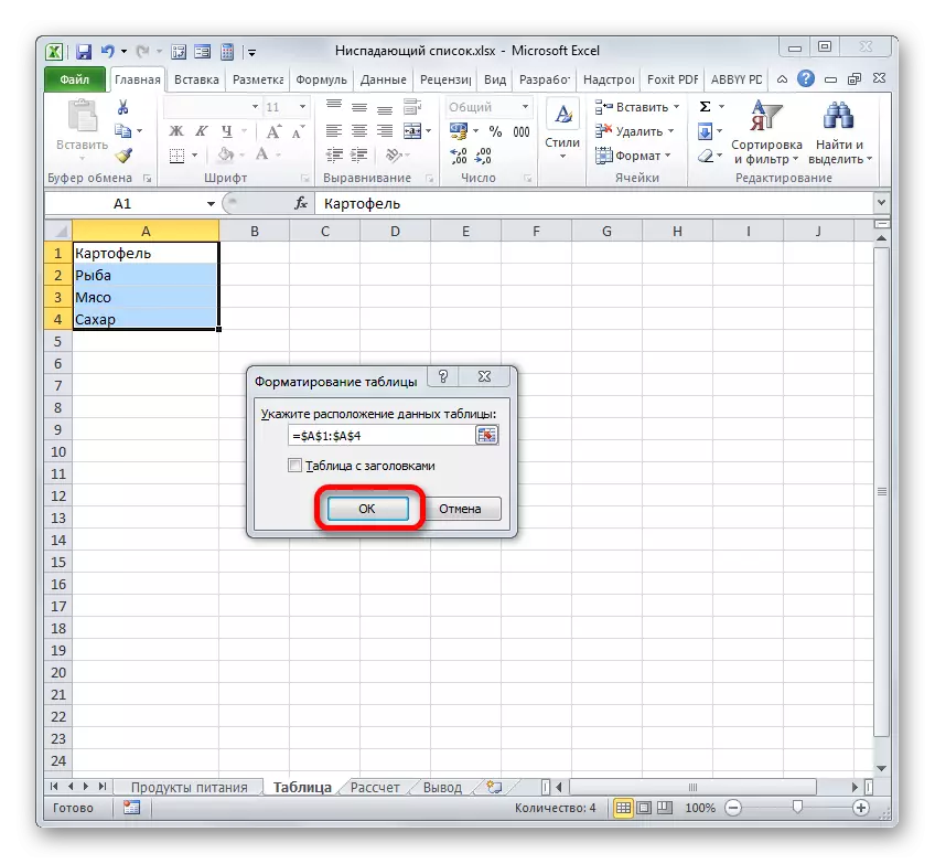
   After that, a small window opens, which contains the address of the selected array. If the selection was performed correctly, then nothing needs to be changed. Since our range has no headers, then the "Table with headlines" item should not be. Although specifically in your case, it is possible, the title will be applied. So we can just click on the "OK" button.

   

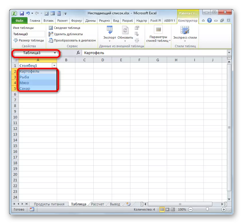
   After that, the range will be formatted as the table. If it is allocated, then you can see in the area of ​​names, that the name he was assigned automatically. This name can be used to insert into the "Source" area in the data verification window according to the previously described algorithm. But, if you want to use another name, you can replace it, just on the names of the name.

   

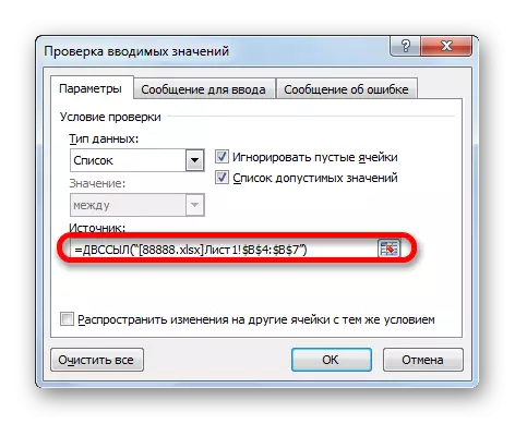
   If the list is posted in another book, then for its correct reflection it is required to apply the function DVSL. The specified operator is intended to form "superabsolite" references to sheet elements in text form. Actually, the procedure will be performed almost exactly the same as in the previously described cases, only in the "Source" area after the symbol "=" should specify the name of the operator - "DVSSL". After that, in brackets, the address of the range must be specified as the argument of this function, including the name of the book and sheet. Actually, as shown in the image below.



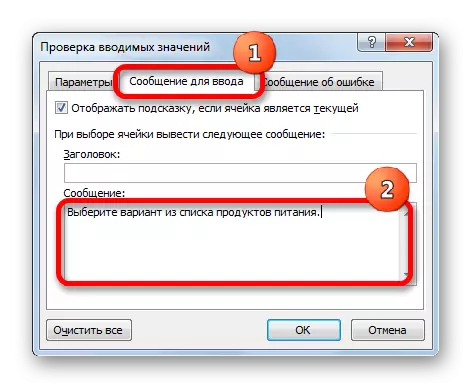
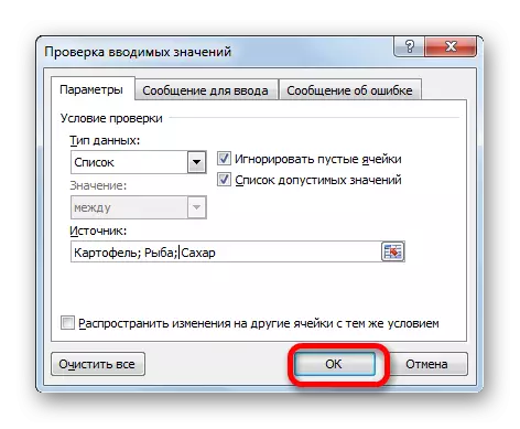
3. On this we could and end the procedure by clicking on the "OK" button in the data verification window, but if you wish, you can improve the form. Go to the "Messages to enter" section of the data verification window. Here in the "Message" area you can write the text that users will see the cursor to the leaf element with a drop-down list. We write down the message that we consider it necessary.



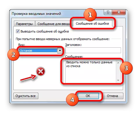
4. Next, we move to the "Error Message" section. Here in the "Message" area, you can enter the text that the user will observe when trying to enter incorrect data, that is, any data that is missing in the drop-down list. In the "View" area, you can select the icon to be accompanied by a warning. Enter the text of the message and clay on "OK".

Lesson: How to make a drop-down list in Excel

Performing operations

Now let's figure it out how to work with the tool that we have created above.

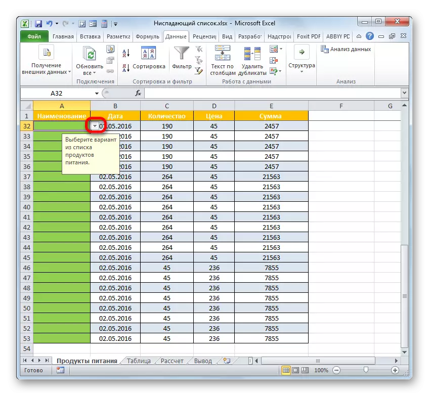
1. If we set the cursor to any leaf element to which the distance has been applied, we will see the informational message introduced by us earlier in the data verification window. In addition, a pictogram in the form of a triangle will appear to the right of the cell. It is it that it serves to access the selection of listing elements. Clay on this triangle.



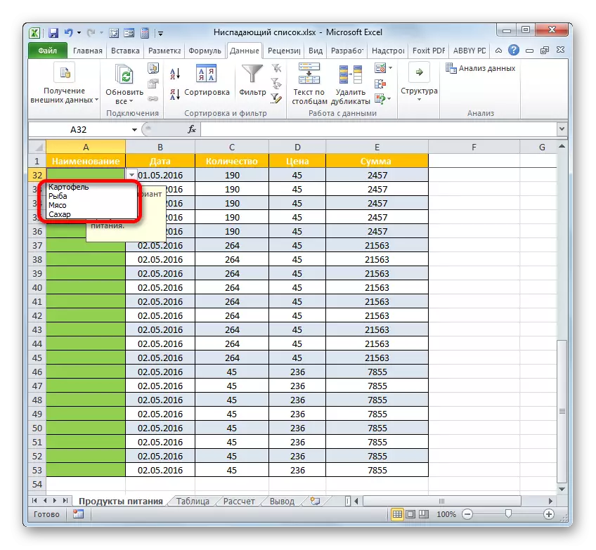
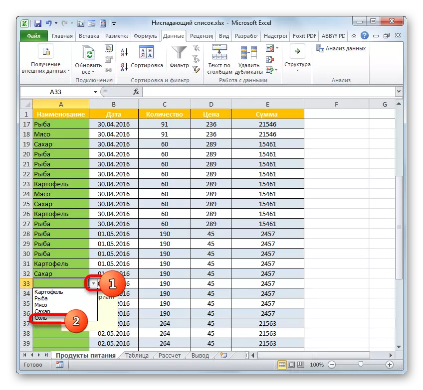
2. After clicking on it, the menu from the list of objects will be open. It contains all items that were previously made through the data verification window. Choose the option that we consider it necessary.



3. The selected option will be displayed in the cell.



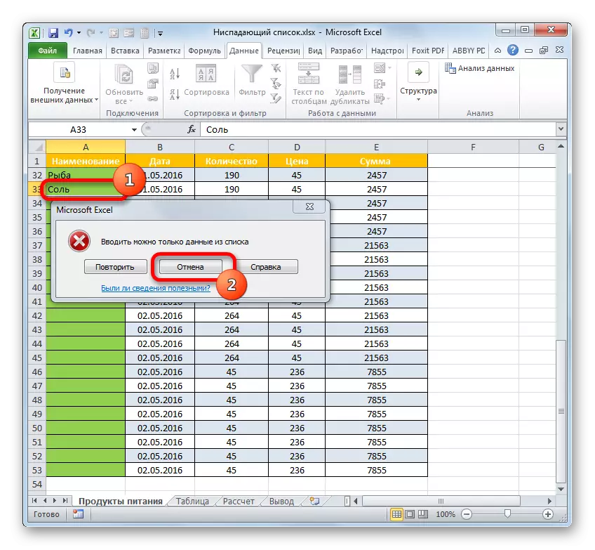
4. If we try to enter into a cell any value that is absent in the list, this action will be blocked. At the same time, if you contributed a warning message to the data verification window, it is displayed on the screen. You need to click on the "Cancel" button in the warning window and with the next attempt to enter correct data.

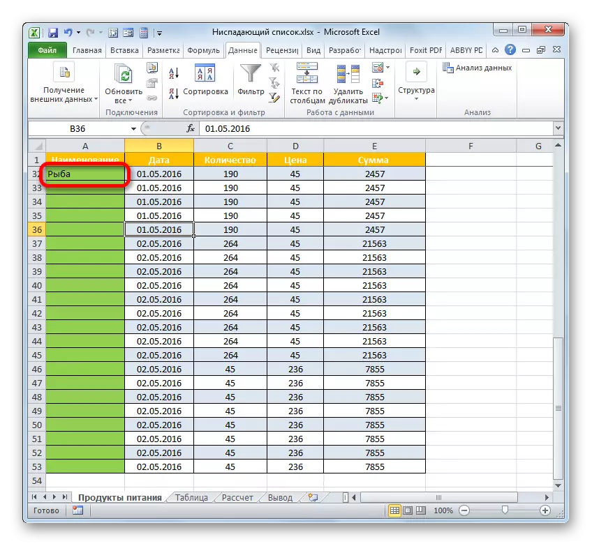
In this way, if necessary, fill the entire table.

Adding a new element

But what should I need to add a new element yet? Actions here depend on how you formed a list in the Data Verification window: Entered manually or pulled up from a table array.

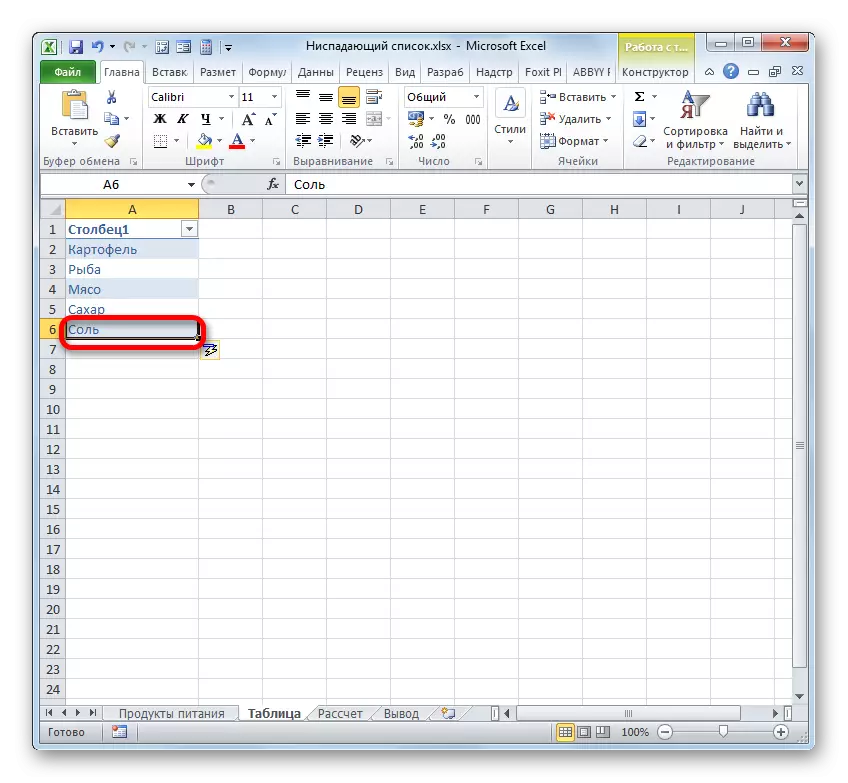
1. If the data for the formation of the list is pulled from a table array, then go to it. Select the range of the range. If this is not a "smart" table, but a simple range of data, then you need to insert a string in the middle of the array. If you apply a "smart" table, then in this case it is enough to just enter the desired value in the first line under it and this line will immediately be included in the table array. This is just the advantage of the "smart" table, which we mentioned above.

   

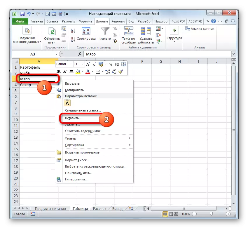
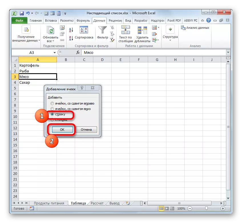
   But suppose we are dealing with a more complex occasion using a regular range. So, we highlight the cell in the middle of the specified array. That is, above this cell and under it there must be more lines of the array. Clay on the designated fragment with the right mouse button. In the menu, select the option "Paste ...".



2. A window starts, where the selection of the insert object should be made. Select the "string" option and click on the "OK" button.



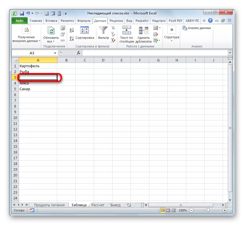
3. So, the empty string is added.



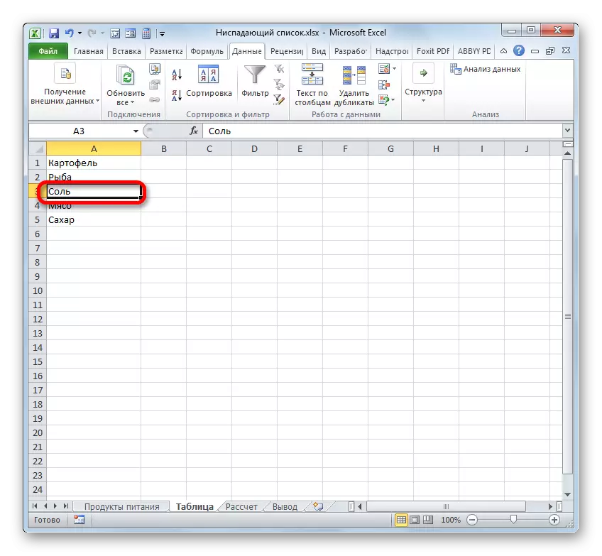
4. Enter the value that we wish to be displayed in the drop-down list.



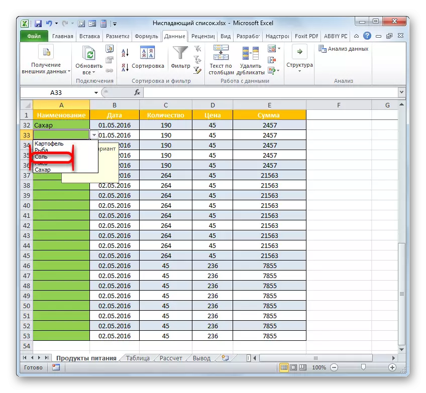
5. After that, we return to the tabletoma array, which places the drop-down list. By clicking on the triangle, to the right of any cell of the array, we see that the value necessary for the already existing list items was added. Now, if you wish, you can choose to insert into the table element.

But what to do if the list of values ​​is tightened not from a separate table, but was made manually? To add an item in this case, also has its own algorithm of action.

1. We highlight the entire table range, in the elements of which the drop-down list is located. Go to the "Data" tab and click on the "Data Verification" button again in the "Work with Data" group.



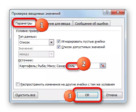
2. The verification window is started. We move to the "Parameters" section. As you can see, all the settings here are exactly the same as we put them earlier. We will be interested in the "source" in this case. We add to the already having a list through a point with a comma (;) the value or the values ​​that we want to see in the drop-down list. After adding clay to "OK".



3. Now, if we open the drop-down list in the table array, we will see a value added there.

Removing item

The removal of the list of the element is carried out at exactly the same algorithm as the addition.

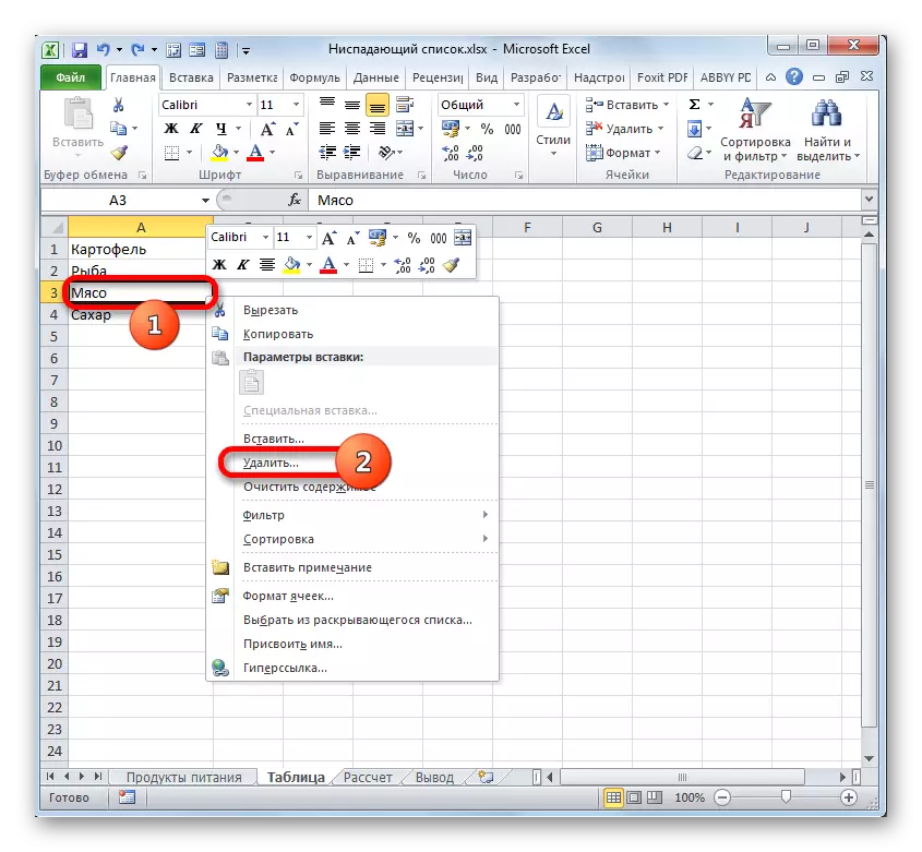
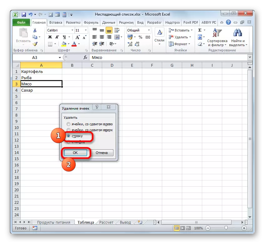
1. If the data is tightened from the table array, then then go to this table and clay right-click on the cell where the value to be deleted is located. In the context menu, stop the choice on the "Delete ..." option.



2. A window removal window is almost similar to the one that we have seen when adding them. Here we set the switch to the "string" position and clay on "OK".



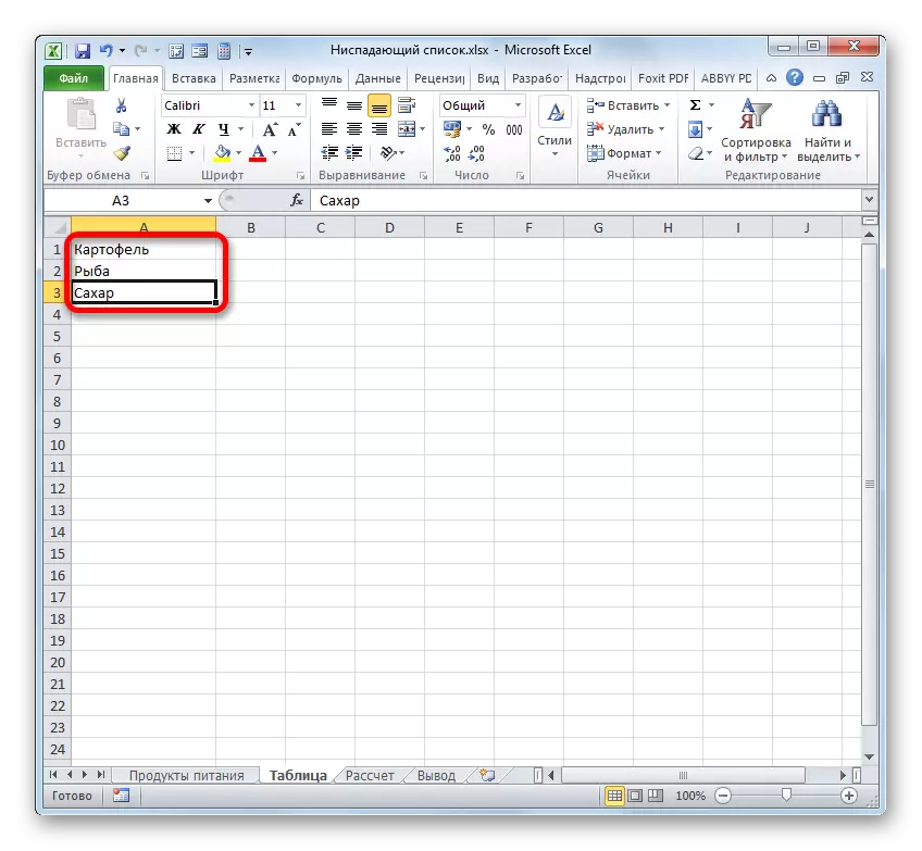
3. A string from a table array, as we can see, deleted.



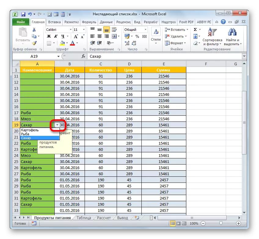
4. Now we return to that table where there are cells with a drop-down list. Clay in the triangle to the right of any cell. In the discontinued list we see that the remote item is absent.

What should I do if the values ​​were added to the data check window manually, and not using an additional table?

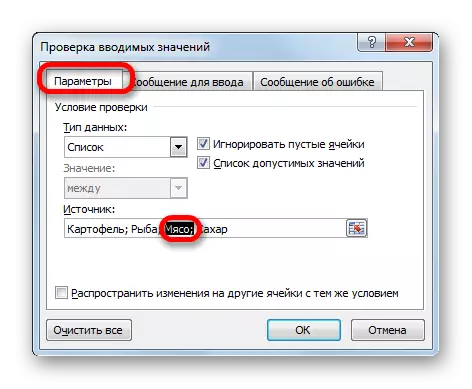
1. We highlight the table with the drop-down list and go to the check box of values, as we have already done earlier. In the specified window, we move to the "Parameters" section. In the "Source" area, we allocate the cursor to the value you want to delete. Then press the Delete button on the keyboard.



2. After the element is removed, click on "OK". Now it will not be in the drop-down list, just as we have seen in the previous version of actions with a table.

Full removal

At the same time, there are situations where the drop-down list needs to be completely removed. If it does not matter that the data entered is saved, then removal is very simple.

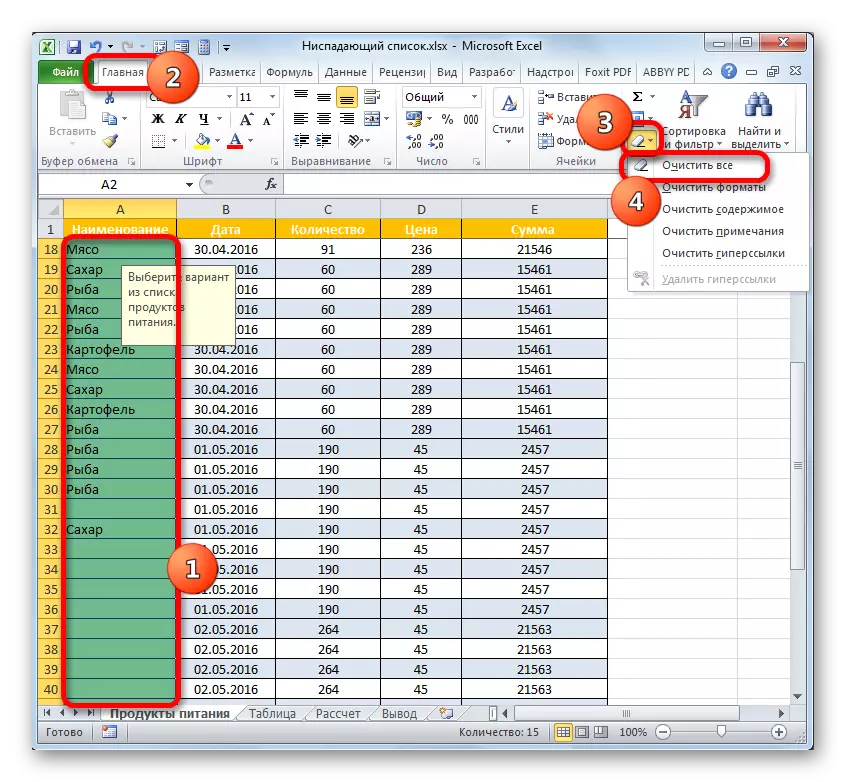
1. We allocate the entire array where the drop-down list is located. Moving to the "Home" tab. Click on the "Clear" icon, which is placed on the ribbon in the Editing unit. In the menu that opens, select the "Clear All" position.



2. When this action is selected in the selected elements of the sheet, all values ​​will be deleted, formatting is cleaned, and the main goal of the task is reached: the drop-down list will be deleted and now you can enter any values ​​manually in the cell.

In addition, if the user does not need to save the entered data, then there is another option to remove the drop-down list.

1. We highlight the range of empty cells, which is equivalent to the range of array elements with the drop-down list. Moving into the "Home" tab and there I click on the "Copy" icon, which is localized on the ribbon in the "Exchange buffer".

   

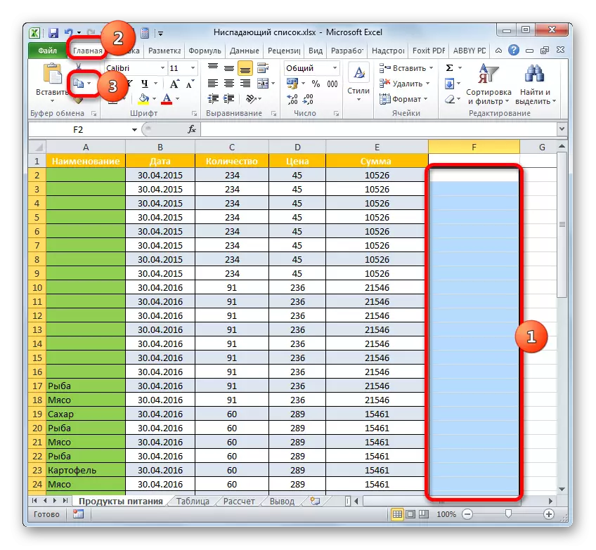
   Also, instead of this action, you can click on the designated fragment by the right mouse button and stop at the "Copy" option.

   

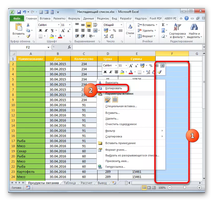
   Even easier immediately after the selection, apply the set of Ctrl + C buttons.

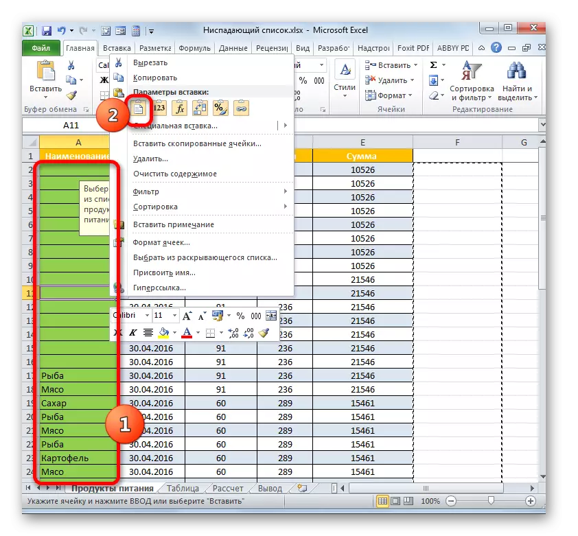
2. After that, we allocate that fragment of the table array, where the drop-down elements are located. We click on the "Insert" button, localized on the tape in the Home tab in the "Exchange Buffer" section.

   

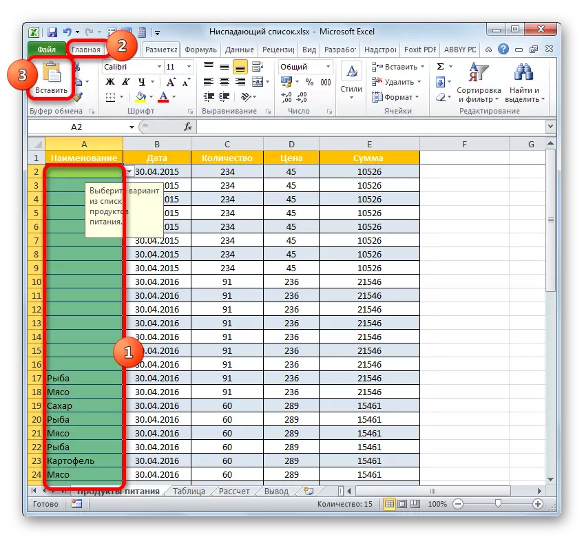
   The second option of actions is to highlight the right mouse button and stop the selection on the "Insert" option in the Insert Parameters group.

   

   Finally, it is possible to simply designate the desired cells and type the combination of the Ctrl + V buttons.

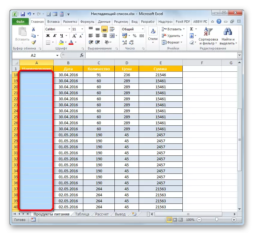
3. With any of the above steps instead of cells containing values ​​and drop-down lists, an absolutely clean fragment will be inserted.

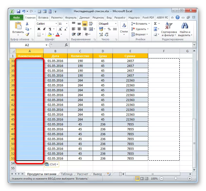
If you wish, you can insert a blank range, but a copied fragment with data. The lack of drop-down lists is that they cannot be manually inserting data missing in the list, but they can be copied and inserted. In this case, the data verification will not work. Moreover, as we found out, the structure of the drop-down list itself will be destroyed.

Often, it is necessary to still remove the drop-down list, but at the same time leaving the values ​​that were introduced using it, and formatting. In this case, more correct steps to remove the specified fill tool are performed.

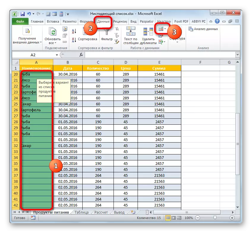
1. We highlight the entire fragment in which elements with the drop-down list are located. Moving to the "Data" tab and clay on the "Data Check" icon, which, as we remember, is located on the tape in the "Working with Data" group.



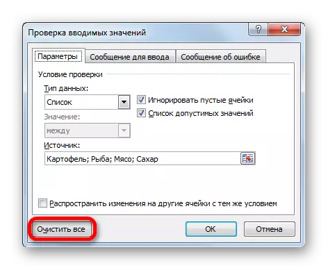
2. A newly familiar test window of the input data opens. Being in any section of the specified tool, we need to make a single action - click on the "Clear All" button. It is located in the lower left corner of the window.



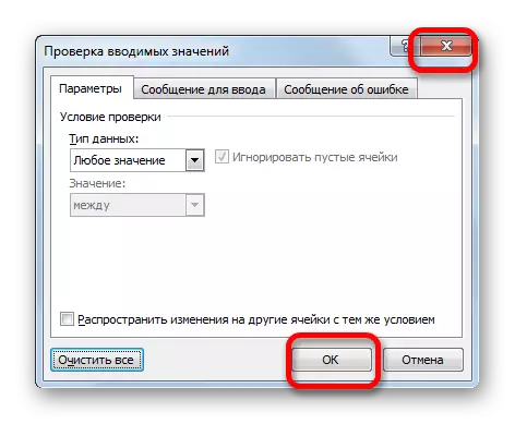
3. After that, the data verification window can be closed by clicking on the standard closing button in its upper right corner as a cross or the "OK" button at the bottom of the window.



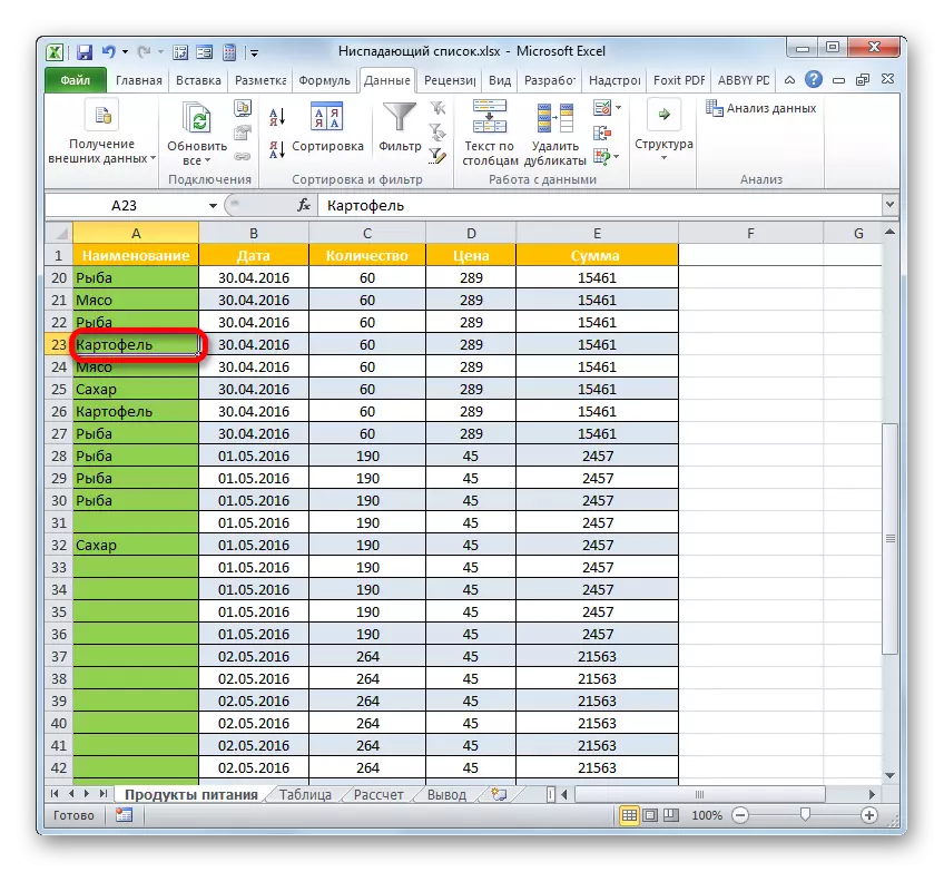
4. Then we allocate any of the cells in which the drop-down list has been placed before. As we see, now there is no hint when selecting an item, nor a triangle to call the list to the right of the cell. But at the same time, formatting remains untouched and all the values ​​entered using the list are left. This means that with the task we coped successfully: a tool that we don't need more, deleted, but the results of his work remained integer.

As you can see, the drop-down list can significantly facilitate the introduction of data into the table, as well as prevent the introduction of incorrect values. This will reduce the number of errors when filling out tables. If you need to add any value additionally, you can always conduct an edit procedure. The editing option will depend on the creation method. After filling in the table, you can delete the drop-down list, although it is not necessary to do this. Most users prefer to leave it even after the end of the table is completed.